Stable Diffusion

Methods

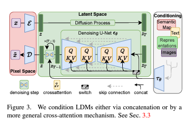
The methodology describes the architecture and training process of Latent Diffusion Models (LDMs):

• The central idea is to perform the diffusion process not in the high-dimensional pixel space but in a compressed latent space. This is achieved by encoding images into a latent space using a pre-trained autoencoder.

Let the encoder and decoder of the autoencoder be denoted by $E(\cdot)$ and $D(\cdot)$, respectively. For an input image $x$, the latent representation $z$ is:

The decoding process reconstructs the image as:

• In Latent Diffusion Models, the denoising process iteratively refines the latent representation instead of raw pixels. This approach greatly reduces dimensionality and computational overhead.

Let $z_t$ denote the noisy latent variable at time step $t$. The forward diffusion process gradually corrupts $z_0$ using a fixed noise schedule:

where $\bar{\alpha}t = \prod{s=1}^{t} \alpha_s$, and $\alpha_t = 1 - \beta_t$, with $\beta_t$ being the variance schedule.

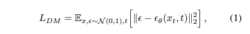
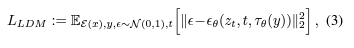
The model learns a denoising function $\epsilon_\theta$ by minimizing the following simplified loss:

This corresponds to learning to predict the noise added at each timestep, conditioned on timestep $t$ and optional text condition $c$.

Algorithmic Flow:

1. Encoding: $z_0 \leftarrow E(x)$
2. Forward Diffusion: Sample $z_t \sim q(z_t | z_0)$
3. Noise Prediction: Predict $\hat{\epsilon} = \epsilon_\theta(z_t, t, c)$
4. Loss Computation: $\mathcal{L} = | \epsilon - \hat{\epsilon} |^2$
5. Denoising (Sampling): At inference, perform reverse steps to generate $\hat{z}_0 \rightarrow \hat{x}$

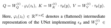
The cross-attention mechanism in the U-Net decoder is defined as:

where $\tau_\theta(y)$ is the text embedding and $\varphi_i(z_t)$ is the intermediate latent representation.

U-Net Architecture

The U-Net serves as the primary denoising network. It uses a convolutional architecture to progressively compress and then reconstruct image features:

• Downsampling path compresses the noisy latent image.
• Upsampling path reconstructs a cleaner image by reversing the downsampling process.
• Skip connections pass high-frequency details across the network.
• Cross-attention layers integrate text embeddings into visual features.

The text condition $c$ is obtained via a text encoder $\tau(\cdot)$, typically a frozen CLIP or transformer model.

Evaluation Metrics

FID Score

The Frechet Inception Distance (FID) is a standard metric for evaluating the realism of generated images. It compares the distribution of generated images to real images using their feature embeddings:

1. Extract image embeddings $\phi(x)$ from real and generated images.
2. Estimate empirical means $\mu_r, \mu_g$ and covariances $\Sigma_r, \Sigma_g$.

FID Formula:

CLIP Score

The CLIP Score evaluates how well the generated image aligns with the input text prompt. CLIP encodes both modalities into a shared embedding space:

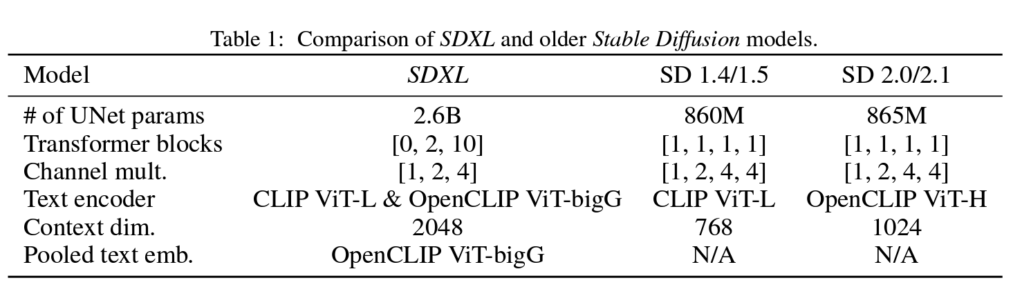
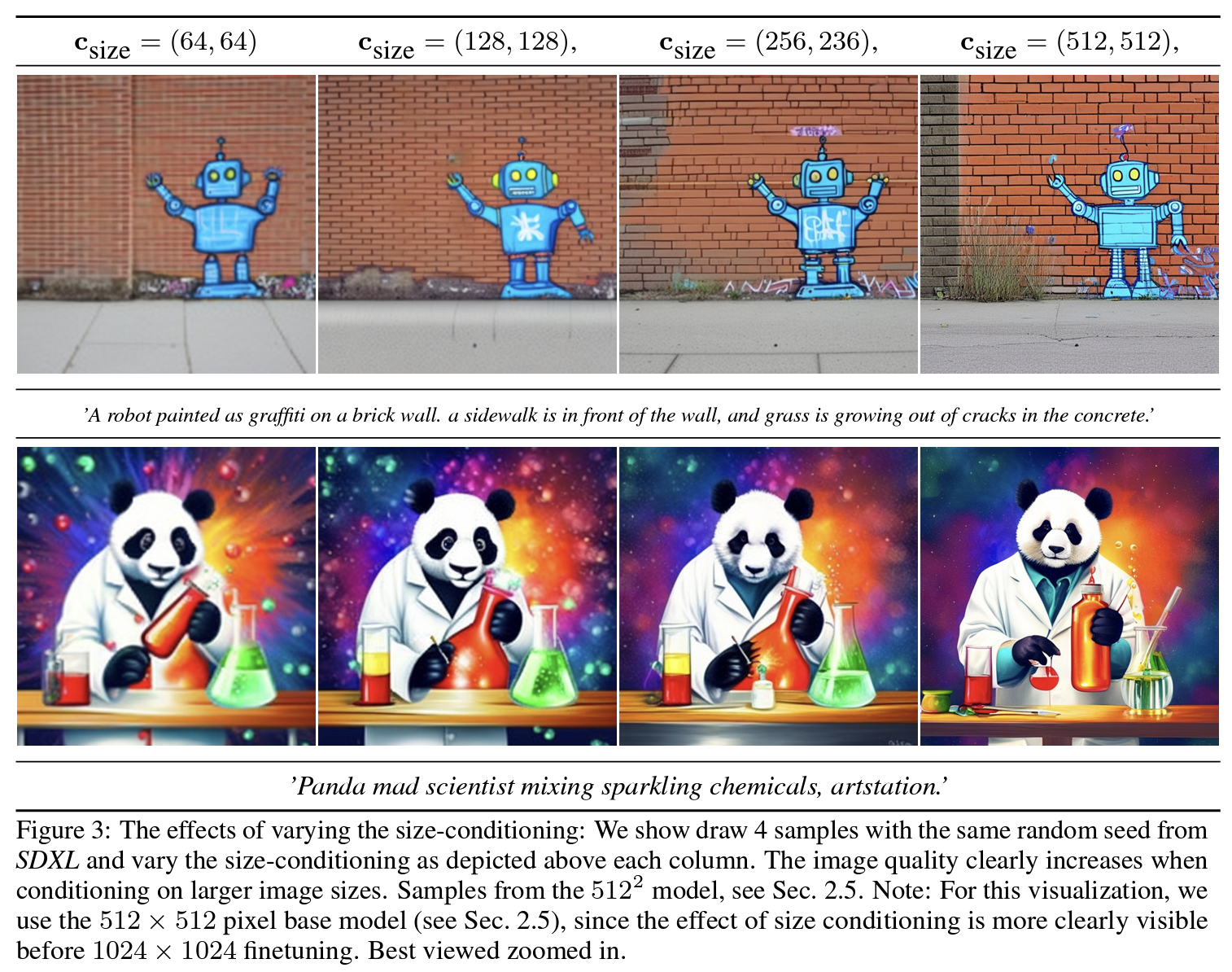
SDXL: Extension of Stable Diffusion

SDXL builds upon Stable Diffusion with architectural and training enhancements:

• Larger U-Net Backbone for richer generation capacity.
• Multi-scale Generation from 512×512 to higher resolutions:

• Flexible Prompt Conditioning:

Conclusion

Stable Diffusion introduced an efficient diffusion framework by operating in latent space, significantly improving speed and scalability.

SDXL pushes this further with architectural depth, better text understanding (OpenCLIP ViT-bigG), and multi-scale generation. It achieves better results in both prompt fidelity (CLIP) and realism (FID).

These models demonstrate the increasing viability of generative models for professional use, spanning art, content creation, and scientific visualization.